


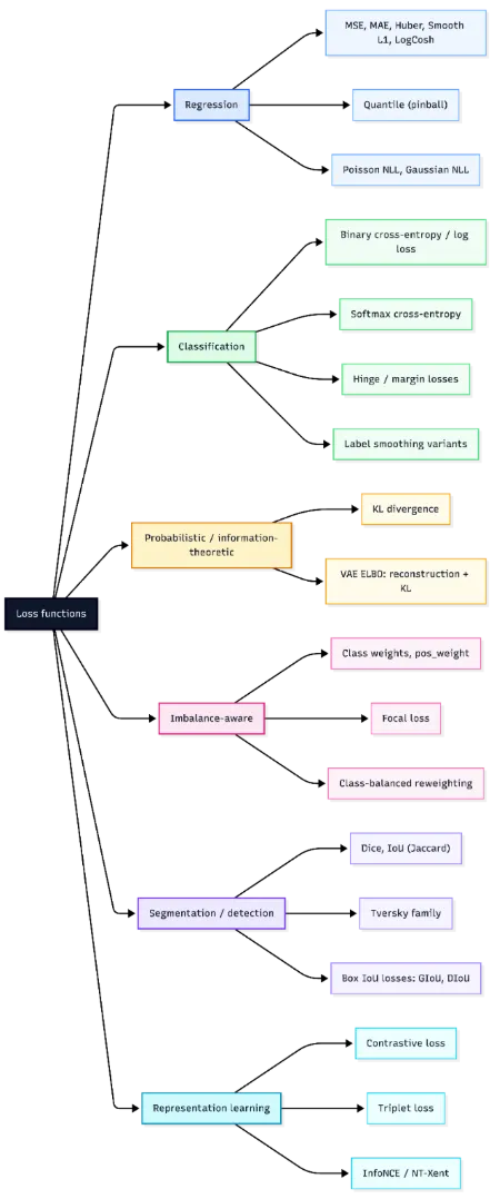
A loss function is what guides a model during training, translating predictions into a signal it can improve on. But not all losses behave the same—some amplify large errors, others stay stable in noisy settings, and each choice subtly shapes how learning unfolds.
Modern libraries add another layer with reduction modes and scaling effects that influence optimization. In this article, we break down the major loss families and how to choose the right one for your task.
Mathematical Foundations of Loss Functions
In supervised learning, the objective is typically to minimize the empirical risk,
(often with optional sample weights and regularization).
where ℓ is the loss function, fθ(xi) is the model prediction, and yi is the true target. In practice, this objective may also include sample weights and regularization terms. Most machine learning frameworks follow this formulation by computing per-example losses and then applying a reduction such as mean, sum, or none.
When discussing mathematical properties, it is important to state the variable with respect to which the loss is analyzed. Many loss functions are convex in the prediction or logit for a fixed label, although the overall training objective is usually non-convex in neural network parameters. Important properties include convexity, differentiability, robustness to outliers, and scale sensitivity. Common implementation of pitfalls includes confusing logits with probabilities and using a reduction that does not match the intended mathematical definition.
Regression Losses
Mean Squared Error
Mean Squared Error, or MSE, is one of the most widely used loss functions for regression. It is defined as the average of the squared differences between predicted values and true targets:
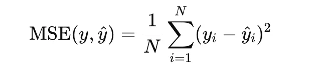
Because the error term is squared, large residuals are penalized more heavily than small ones. This makes MSE useful when large prediction errors should be strongly discouraged. It is convex in the prediction and differentiable everywhere, which makes optimization straightforward. However, it is sensitive to outliers, since a single extreme residual can strongly affect the loss.
import numpy as np
import matplotlib.pyplot as plt

y_true = np.array([3.0, -0.5, 2.0, 7.0])
y_pred = np.array([2.5, 0.0, 2.0, 8.0])

mse = np.mean((y_true - y_pred) ** 2)
print("MSE:", mse)
Mean Absolute Error
Mean Absolute Error, or MAE, measures the average absolute difference between predictions and targets:
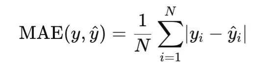
Unlike MSE, MAE penalizes errors linearly rather than quadratically. As a result, it is more robust to outliers. MAE is convex in the prediction, but it is not differentiable at zero residual, so optimization typically uses subgradients at that point.
import numpy as np

y_true = np.array([3.0, -0.5, 2.0, 7.0])
y_pred = np.array([2.5, 0.0, 2.0, 8.0])

mae = np.mean(np.abs(y_true - y_pred))

print("MAE:", mae)
Huber Loss
Huber loss combines the strengths of MSE and MAE by behaving quadratically for small errors and linearly for large ones. For a threshold δ>0, it is defined as:
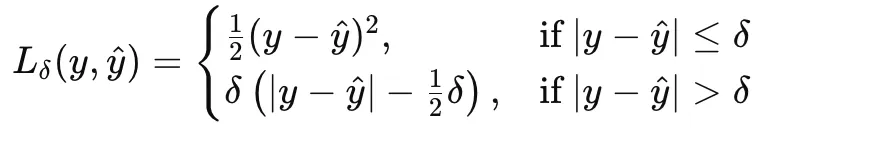
This makes Huber loss a good choice when the data are mostly well behaved but may contain occasional outliers.
import numpy as np

y_true = np.array([3.0, -0.5, 2.0, 7.0])
y_pred = np.array([2.5, 0.0, 2.0, 8.0])

error = y_pred - y_true
delta = 1.0

huber = np.mean(
    np.where(
        np.abs(error) <= delta,
        0.5 * error**2,
        delta * (np.abs(error) - 0.5 * delta)
    )
)

print("Huber Loss:", huber)
Smooth L1 Loss
Smooth L1 loss is closely related to Huber loss and is commonly used in deep learning, especially in object detection and regression heads. It transitions from a squared penalty near zero to an absolute penalty beyond a threshold. It is differentiable everywhere and less sensitive to outliers than MSE.
import torch
import torch.nn.functional as F

y_true = torch.tensor([3.0, -0.5, 2.0, 7.0])
y_pred = torch.tensor([2.5, 0.0, 2.0, 8.0])

smooth_l1 = F.smooth_l1_loss(y_pred, y_true, beta=1.0)

print("Smooth L1 Loss:", smooth_l1.item())
Log-Cosh Loss
Log-cosh loss is a smooth alternative to MAE and is defined as
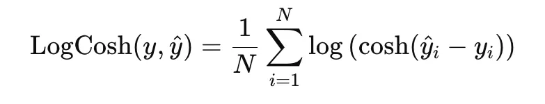
Near zero residuals, it behaves like squared loss, while for large residuals it grows almost linearly. This gives it a good balance between smooth optimization and robustness to outliers.
import numpy as np

y_true = np.array([3.0, -0.5, 2.0, 7.0])
y_pred = np.array([2.5, 0.0, 2.0, 8.0])

error = y_pred - y_true

logcosh = np.mean(np.log(np.cosh(error)))

print("Log-Cosh Loss:", logcosh)
Quantile Loss
Quantile loss, also called pinball loss, is used when the goal is to estimate a conditional quantile rather than a conditional mean. For a quantile level τ∈(0,1) and residual u=y−y^ it is defined as
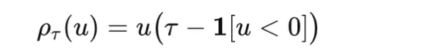
It penalizes overestimation and underestimation asymmetrically, making it useful in forecasting and uncertainty estimation.
import numpy as np

y_true = np.array([3.0, -0.5, 2.0, 7.0])
y_pred = np.array([2.5, 0.0, 2.0, 8.0])

tau = 0.8

u = y_true - y_pred

quantile_loss = np.mean(np.where(u >= 0, tau * u, (tau - 1) * u))

print("Quantile Loss:", quantile_loss)
import numpy as np

y_true = np.array([3.0, -0.5, 2.0, 7.0])
y_pred = np.array([2.5, 0.0, 2.0, 8.0])

tau = 0.8

u = y_true - y_pred

quantile_loss = np.mean(np.where(u >= 0, tau * u, (tau - 1) * u))

print("Quantile Loss:", quantile_loss)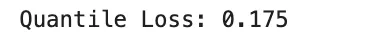
MAPE
Mean Absolute Percentage Error, or MAPE, measures relative error and is defined as
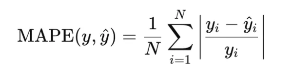
It is useful when relative error matters more than absolute error, but it becomes unstable when target values are zero or very close to zero.
import numpy as np

y_true = np.array([100.0, 200.0, 300.0])
y_pred = np.array([90.0, 210.0, 290.0])

mape = np.mean(np.abs((y_true - y_pred) / y_true))

print("MAPE:", mape)
MSLE
Mean Squared Logarithmic Error, or MSLE, is defined as
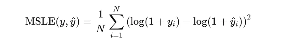
It is useful when relative differences matter and the targets are nonnegative.
import numpy as np

y_true = np.array([100.0, 200.0, 300.0])
y_pred = np.array([90.0, 210.0, 290.0])

msle = np.mean((np.log1p(y_true) - np.log1p(y_pred)) ** 2)

print("MSLE:", msle)
Poisson Negative Log-Likelihood
Poisson negative log-likelihood is used for count data. For a rate parameter λ>0, it is typically written as
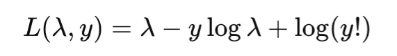
In practice, the constant term may be omitted. This loss is appropriate when targets represent counts generated from a Poisson process.
import numpy as np

y_true = np.array([2.0, 0.0, 4.0])
lam = np.array([1.5, 0.5, 3.0])

poisson_nll = np.mean(lam - y_true * np.log(lam))

print("Poisson NLL:", poisson_nll)
Gaussian Negative Log-Likelihood
Gaussian negative log-likelihood allows the model to predict both the mean and the variance of the target distribution. A common form is
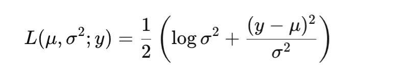
This is useful for heteroscedastic regression, where the noise level varies across inputs.
import numpy as np

y_true = np.array([0.0, 1.0])
mu = np.array([0.0, 1.5])
var = np.array([1.0, 0.25])

gaussian_nll = np.mean(0.5 * (np.log(var) + (y_true - mu) ** 2 / var))

print("Gaussian NLL:", gaussian_nll)
Classification and Probabilistic Losses
Binary Cross-Entropy and Log Loss
Binary cross-entropy, or BCE, is used for binary classification. It compares a Bernoulli label y∈{0,1} with a predicted probability p∈(0,1):
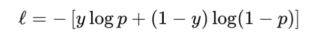
In practice, many libraries prefer logits rather than probabilities and compute the loss in a numerically stable way. This avoids instability caused by applying sigmoid separately before the logarithm. BCE is convex in the logit for a fixed label and differentiable, but it is not robust to label noise because confidently wrong predictions can produce very large loss values. It is widely used for binary classification, and in multi-label classification it is applied independently to each label. A common pitfall is confusing probabilities with logits, which can silently degrade training.
import torch

logits = torch.tensor([2.0, -1.0, 0.0])
y_true = torch.tensor([1.0, 0.0, 1.0])

bce = torch.nn.BCEWithLogitsLoss()
loss = bce(logits, y_true)

print("BCEWithLogitsLoss:", loss.item())
Softmax Cross-Entropy for Multiclass Classification
Softmax cross-entropy is the standard loss for multiclass classification. For a class index y and logits vector z, it combines the softmax transformation with cross-entropy loss:
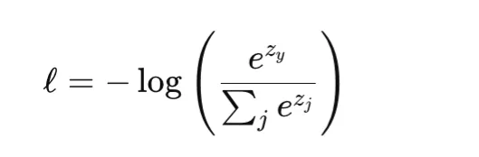
This loss is convex in the logits and differentiable. Like BCE, it can heavily penalize confident wrong predictions and is not inherently robust to label noise. It is commonly used in standard multiclass classification and also in pixelwise classification tasks such as semantic segmentation. One important implementation detail is that many libraries, including PyTorch, expect integer class indices rather than one-hot targets unless soft-label variants are explicitly used.
import torch
import torch.nn.functional as F

logits = torch.tensor([
    [2.0, 0.5, -1.0],
    [0.0, 1.0, 0.0]
], dtype=torch.float32)

y_true = torch.tensor([0, 2], dtype=torch.long)

loss = F.cross_entropy(logits, y_true)

print("CrossEntropyLoss:", loss.item())
Label Smoothing Variant
Label smoothing is a regularized form of cross-entropy in which a one-hot target is replaced by a softened target distribution. Instead of assigning full probability mass to the correct class, a small portion is distributed across the remaining classes. This discourages overconfident predictions and can improve calibration.
The method remains differentiable and often improves generalization, especially in large-scale classification. However, too much smoothing can make the targets overly ambiguous and lead to underfitting.
import torch
import torch.nn.functional as F

logits = torch.tensor([
    [2.0, 0.5, -1.0],
    [0.0, 1.0, 0.0]
], dtype=torch.float32)

y_true = torch.tensor([0, 2], dtype=torch.long)

loss = F.cross_entropy(logits, y_true, label_smoothing=0.1)

print("CrossEntropyLoss with label smoothing:", loss.item())
Margin Losses: Hinge Loss
Hinge loss is a classic margin-based loss used in support vector machines. For binary classification with label y∈{−1,+1} and score s, it is defined as
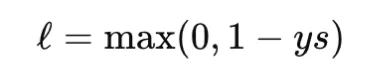
Hinge loss is convex in the score but not differentiable at the margin boundary. It produces zero loss for examples that are correctly classified with sufficient margin, which leads to sparse gradients. Unlike cross-entropy, hinge loss is not probabilistic and does not directly provide calibrated probabilities. It is useful when a max-margin property is desired.
import numpy as np

y_true = np.array([1.0, -1.0, 1.0])
scores = np.array([0.2, 0.4, 1.2])

hinge_loss = np.mean(np.maximum(0, 1 - y_true * scores))

print("Hinge Loss:", hinge_loss)
KL Divergence
Kullback-Leibler divergence compares two probability distributions P and Q:
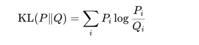
It is nonnegative and becomes zero only when the two distributions are identical. KL divergence is not symmetric, so it is not a true metric. It is widely used in knowledge distillation, variational inference, and regularization of learned distributions toward a prior. In practice, PyTorch expects the input distribution in log-probability form, and using the wrong reduction can change the reported value. In particular, batchmean matches the mathematical KL definition more closely than mean.
import torch
import torch.nn.functional as F

P = torch.tensor([[0.7, 0.2, 0.1]], dtype=torch.float32)
Q = torch.tensor([[0.6, 0.3, 0.1]], dtype=torch.float32)

kl_batchmean = F.kl_div(Q.log(), P, reduction="batchmean")

print("KL Divergence (batchmean):", kl_batchmean.item())
KL Divergence Reduction Pitfall
A common implementation issue with KL divergence is the choice of reduction. In PyTorch, reduction=”mean” scales the result differently from the true KL expression, while reduction=”batchmean” better matches the standard definition.
import torch
import torch.nn.functional as F

P = torch.tensor([[0.7, 0.2, 0.1]], dtype=torch.float32)
Q = torch.tensor([[0.6, 0.3, 0.1]], dtype=torch.float32)

kl_batchmean = F.kl_div(Q.log(), P, reduction="batchmean")
kl_mean = F.kl_div(Q.log(), P, reduction="mean")

print("KL batchmean:", kl_batchmean.item())
print("KL mean:", kl_mean.item())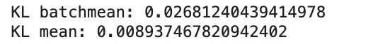
Variational Autoencoder ELBO
The variational autoencoder, or VAE, is trained by maximizing the evidence lower bound, commonly called the ELBO:
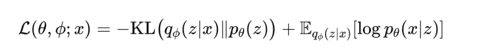
This objective has two parts. The reconstruction term encourages the model to explain the data well, while the KL term regularizes the approximate posterior toward the prior. The ELBO is not convex in neural network parameters, but it is differentiable under the reparameterization trick. It is widely used in generative modeling and probabilistic representation learning. In practice, many variants introduce a weight on the KL term, such as in beta-VAE.
import torch

reconstruction_loss = torch.tensor(12.5)
kl_term = torch.tensor(3.2)

elbo = reconstruction_loss + kl_term

print("VAE-style total loss:", elbo.item())
Imbalance-Aware Losses
Class Weights
Class weighting is a common strategy for handling imbalanced datasets. Instead of treating all classes equally, higher loss weight is assigned to minority classes so that their errors contribute more strongly during training. In multiclass classification, weighted cross-entropy is often used:
where wy is the weight for the true class. This approach is simple and effective when class frequencies differ substantially. However, excessively large weights can make optimization unstable.
import torch
import torch.nn.functional as F

logits = torch.tensor([
    [2.0, 0.5, -1.0],
    [0.0, 1.0, 0.0],
    [0.2, -0.1, 1.5]
], dtype=torch.float32)

y_true = torch.tensor([0, 1, 2], dtype=torch.long)
class_weights = torch.tensor([1.0, 2.0, 3.0], dtype=torch.float32)

loss = F.cross_entropy(logits, y_true, weight=class_weights)

print("Weighted Cross-Entropy:", loss.item())
Positive Class Weight for Binary Loss
For binary or multi-label classification, many libraries provide a pos_weight parameter that increases the contribution of positive examples in binary cross-entropy. This is especially useful when positive labels are rare. In PyTorch, BCEWithLogitsLoss supports this directly.
This method is often preferred over naive resampling because it preserves all examples while adjusting the optimization signal. A common mistake is to confuse weight and pos_weight, since they affect the loss differently.
import torch

logits = torch.tensor([2.0, -1.0, 0.5], dtype=torch.float32)
y_true = torch.tensor([1.0, 0.0, 1.0], dtype=torch.float32)

criterion = torch.nn.BCEWithLogitsLoss(pos_weight=torch.tensor([3.0]))
loss = criterion(logits, y_true)

print("BCEWithLogitsLoss with pos_weight:", loss.item())
Focal Loss
Focal loss is designed to address class imbalance by down-weighting easy examples and focusing training on harder ones. For binary classification, it is commonly written as
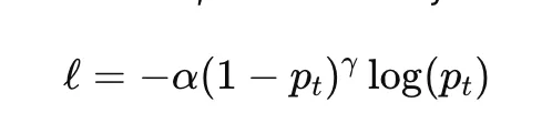
where pt is the model probability assigned to the true class, α is a class-balancing factor, and γ controls how strongly easy examples are down-weighted. When γ=0, focal loss reduces to ordinary cross-entropy.
Focal loss is widely used in dense object detection and highly imbalanced classification problems. Its main hyperparameters are α and γ, both of which can significantly affect training behavior.
import torch
import torch.nn.functional as F

logits = torch.tensor([2.0, -1.0, 0.5], dtype=torch.float32)
y_true = torch.tensor([1.0, 0.0, 1.0], dtype=torch.float32)

bce = F.binary_cross_entropy_with_logits(logits, y_true, reduction="none")

probs = torch.sigmoid(logits)
pt = torch.where(y_true == 1, probs, 1 - probs)

alpha = 0.25
gamma = 2.0

focal_loss = (alpha * (1 - pt) ** gamma * bce).mean()

print("Focal Loss:", focal_loss.item())
Class-Balanced Reweighting
Class-balanced reweighting improves on simple inverse-frequency weighting by using the effective number of samples rather than raw counts. A common formula for the class weight is
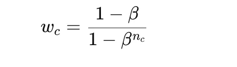
where nc is the number of samples in class c and β is a parameter close to 1. This gives smoother and often more stable reweighting than direct inverse counts.
This method is useful when class imbalance is severe but naive class weights would be too extreme. The main hyperparameter is β, which determines how strongly rare classes are emphasized.
import numpy as np

class_counts = np.array([1000, 100, 10], dtype=np.float64)
beta = 0.999

effective_num = 1.0 - np.power(beta, class_counts)
class_weights = (1.0 - beta) / effective_num

class_weights = class_weights / class_weights.sum() * len(class_counts)

print("Class-Balanced Weights:", class_weights)
Segmentation and Detection Losses
Dice Loss
Dice loss is widely used in image segmentation, especially when the target region is small relative to the background. It is based on the Dice coefficient, which measures overlap between the predicted mask and the ground-truth mask:
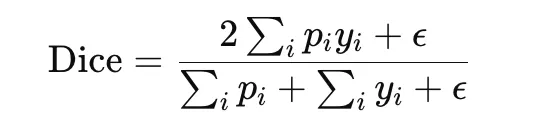
The corresponding loss is
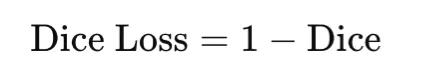
Dice loss directly optimizes overlap and is therefore well suited to imbalanced segmentation tasks. It is differentiable when soft predictions are used, but it can be sensitive to small denominators, so a smoothing constant ϵ is usually added.
import torch

y_true = torch.tensor([1, 1, 0, 0], dtype=torch.float32)
y_pred = torch.tensor([0.9, 0.8, 0.2, 0.1], dtype=torch.float32)

eps = 1e-6

intersection = torch.sum(y_pred * y_true)
dice = (2 * intersection + eps) / (torch.sum(y_pred) + torch.sum(y_true) + eps)

dice_loss = 1 - dice

print("Dice Loss:", dice_loss.item())
IoU Loss
Intersection over Union, or IoU, also called Jaccard index, is another overlap-based measure commonly used in segmentation and detection. It is defined as
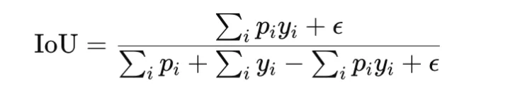
The loss form is
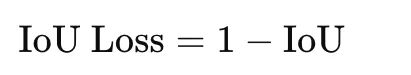
IoU loss is stricter than Dice loss because it penalizes disagreement more strongly. It is useful when accurate region overlap is the main objective. As with Dice loss, a small constant is added for stability.
import torch

y_true = torch.tensor([1, 1, 0, 0], dtype=torch.float32)
y_pred = torch.tensor([0.9, 0.8, 0.2, 0.1], dtype=torch.float32)

eps = 1e-6

intersection = torch.sum(y_pred * y_true)
union = torch.sum(y_pred) + torch.sum(y_true) - intersection

iou = (intersection + eps) / (union + eps)
iou_loss = 1 - iou

print("IoU Loss:", iou_loss.item())
Tversky Loss
Tversky loss generalizes Dice and IoU style overlap losses by weighting false positives and false negatives differently. The Tversky index is
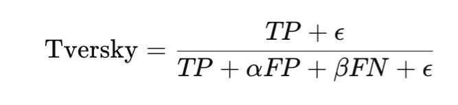
and the loss is
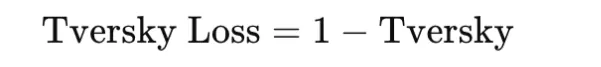
This makes it especially useful in highly imbalanced segmentation problems, such as medical imaging, where missing a positive region may be much worse than including extra background. The choice of α and β controls this tradeoff.
import torch

y_true = torch.tensor([1, 1, 0, 0], dtype=torch.float32)
y_pred = torch.tensor([0.9, 0.8, 0.2, 0.1], dtype=torch.float32)

eps = 1e-6
alpha = 0.3
beta = 0.7

tp = torch.sum(y_pred * y_true)
fp = torch.sum(y_pred * (1 - y_true))
fn = torch.sum((1 - y_pred) * y_true)

tversky = (tp + eps) / (tp + alpha * fp + beta * fn + eps)
tversky_loss = 1 - tversky

print("Tversky Loss:", tversky_loss.item())
Generalized IoU Loss
Generalized IoU, or GIoU, is an extension of IoU designed for bounding-box regression in object detection. Standard IoU becomes zero when two boxes do not overlap, which gives no useful gradient. GIoU addresses this by incorporating the smallest enclosing box CCC:
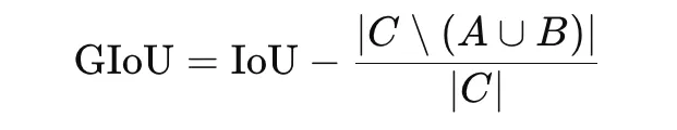
The loss is

GIoU is useful because it still provides a training signal even when predicted and true boxes do not overlap.
import torch

def box_area(box):
    return max(0.0, box[2] - box[0]) * max(0.0, box[3] - box[1])

def intersection_area(box1, box2):
    x1 = max(box1[0], box2[0])
    y1 = max(box1[1], box2[1])
    x2 = min(box1[2], box2[2])
    y2 = min(box1[3], box2[3])
    return max(0.0, x2 - x1) * max(0.0, y2 - y1)

pred_box = [1.0, 1.0, 3.0, 3.0]
true_box = [2.0, 2.0, 4.0, 4.0]

inter = intersection_area(pred_box, true_box)
area_pred = box_area(pred_box)
area_true = box_area(true_box)

union = area_pred + area_true - inter
iou = inter / union

c_box = [
    min(pred_box[0], true_box[0]),
    min(pred_box[1], true_box[1]),
    max(pred_box[2], true_box[2]),
    max(pred_box[3], true_box[3]),
]

area_c = box_area(c_box)
giou = iou - (area_c - union) / area_c

giou_loss = 1 - giou

print("GIoU Loss:", giou_loss)
Distance IoU Loss
Distance IoU, or DIoU, extends IoU by adding a penalty based on the distance between box centers. It is defined as
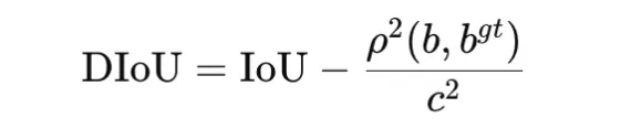
where ρ2(b,bgt) is the squared distance between the centers of the predicted and ground-truth boxes, and c2 is the squared diagonal length of the smallest enclosing box. The loss is
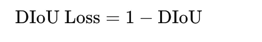
DIoU improves optimization by encouraging both overlap and spatial alignment. It is commonly used in bounding-box regression for object detection.
import math

def box_center(box):
    return ((box[0] + box[2]) / 2.0, (box[1] + box[3]) / 2.0)

def intersection_area(box1, box2):
    x1 = max(box1[0], box2[0])
    y1 = max(box1[1], box2[1])
    x2 = min(box1[2], box2[2])
    y2 = min(box1[3], box2[3])
    return max(0.0, x2 - x1) * max(0.0, y2 - y1)

pred_box = [1.0, 1.0, 3.0, 3.0]
true_box = [2.0, 2.0, 4.0, 4.0]

inter = intersection_area(pred_box, true_box)

area_pred = (pred_box[2] - pred_box[0]) * (pred_box[3] - pred_box[1])
area_true = (true_box[2] - true_box[0]) * (true_box[3] - true_box[1])

union = area_pred + area_true - inter
iou = inter / union

cx1, cy1 = box_center(pred_box)
cx2, cy2 = box_center(true_box)

center_dist_sq = (cx1 - cx2) ** 2 + (cy1 - cy2) ** 2

c_x1 = min(pred_box[0], true_box[0])
c_y1 = min(pred_box[1], true_box[1])
c_x2 = max(pred_box[2], true_box[2])
c_y2 = max(pred_box[3], true_box[3])

diag_sq = (c_x2 - c_x1) ** 2 + (c_y2 - c_y1) ** 2

diou = iou - center_dist_sq / diag_sq
diou_loss = 1 - diou

print("DIoU Loss:", diou_loss)
Representation Learning Losses
Contrastive Loss
Contrastive loss is used to learn embeddings by bringing similar samples closer together and pushing dissimilar samples farther apart. It is commonly used in Siamese networks. For a pair of embeddings with distance d and label y∈{0,1}, where y=1 indicates a similar pair, a common form is
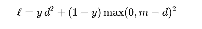
where m is the margin. This loss encourages similar pairs to have small distance and dissimilar pairs to be separated by at least the margin. It is useful in face verification, signature matching, and metric learning.
import torch
import torch.nn.functional as F

z1 = torch.tensor([[1.0, 2.0]], dtype=torch.float32)
z2 = torch.tensor([[1.5, 2.5]], dtype=torch.float32)

label = torch.tensor([1.0], dtype=torch.float32)  # 1 = similar, 0 = dissimilar

distance = F.pairwise_distance(z1, z2)

margin = 1.0

contrastive_loss = (
    label * distance.pow(2)
    + (1 - label) * torch.clamp(margin - distance, min=0).pow(2)
)

print("Contrastive Loss:", contrastive_loss.mean().item())
Triplet Loss
Triplet loss extends pairwise learning by using three examples: an anchor, a positive sample from the same class, and a negative sample from a different class. The objective is to make the anchor closer to the positive than to the negative by at least a margin:
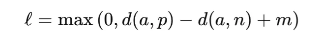
where d(⋅, ⋅) is a distance function and m is the margin. Triplet loss is widely used in face recognition, person re-identification, and retrieval of tasks. Its success depends strongly on how informative triplets are selected during training.
import torch
import torch.nn.functional as F

anchor = torch.tensor([[1.0, 2.0]], dtype=torch.float32)
positive = torch.tensor([[1.1, 2.1]], dtype=torch.float32)
negative = torch.tensor([[3.0, 4.0]], dtype=torch.float32)

margin = 1.0

triplet = torch.nn.TripletMarginLoss(margin=margin, p=2)
loss = triplet(anchor, positive, negative)

print("Triplet Loss:", loss.item())
InfoNCE and NT-Xent Loss
InfoNCE is a contrastive objective widely used in self-supervised representation learning. It encourages an anchor embedding to be close to its positive pair while being far from other samples in the batch, which act as negatives. A standard form is
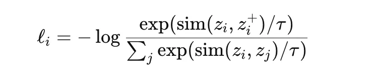
where sim is a similarity measure such as cosine similarity and τ is a temperature parameter. NT-Xent is a normalized temperature-scaled variant commonly used in methods such as SimCLR. These losses are powerful because they learn rich representations without manual labels, but they depend strongly on batch composition, augmentation strategy, and temperature choice.
import torch
import torch.nn.functional as F

z_anchor = torch.tensor([[1.0, 0.0]], dtype=torch.float32)
z_positive = torch.tensor([[0.9, 0.1]], dtype=torch.float32)
z_negative1 = torch.tensor([[0.0, 1.0]], dtype=torch.float32)
z_negative2 = torch.tensor([[-1.0, 0.0]], dtype=torch.float32)

embeddings = torch.cat([z_positive, z_negative1, z_negative2], dim=0)

z_anchor = F.normalize(z_anchor, dim=1)
embeddings = F.normalize(embeddings, dim=1)

similarities = torch.matmul(z_anchor, embeddings.T).squeeze(0)

temperature = 0.1
logits = similarities / temperature

labels = torch.tensor([0], dtype=torch.long)  # positive is first

loss = F.cross_entropy(logits.unsqueeze(0), labels)

print("InfoNCE / NT-Xent Loss:", loss.item())
Comparison Table and Practical Guidance
The table below summarizes key properties of commonly used loss functions. Here, convexity refers to convexity with respect to the model output, such as prediction or logit, for fixed targets, not convexity in neural network parameters. This distinction is important because most deep learning objectives are non-convex in parameters, even when the loss is convex in the output.
| Loss | Typical Task | Convex in Output | Differentiable | Robust to Outliers | Scale / Units |
|---|---|---|---|---|---|
| MSE | Regression | Yes | Yes | No | Squared target units |
| MAE | Regression | Yes | No (kink) | Yes | Target units |
| Huber | Regression | Yes | Yes | Yes (controlled by δ) | Target units |
| Smooth L1 | Regression / Detection | Yes | Yes | Yes | Target units |
| Log-cosh | Regression | Yes | Yes | Moderate | Target units |
| Pinball (Quantile) | Regression / Forecast | Yes | No (kink) | Yes | Target units |
| Poisson NLL | Count Regression | Yes (λ>0) | Yes | Not primary focus | Nats |
| Gaussian NLL | Uncertainty Regression | Yes (mean) | Yes | Not primary focus | Nats |
| BCE (logits) | Binary / Multilabel | Yes | Yes | Not applicable | Nats |
| Softmax Cross-Entropy | Multiclass | Yes | Yes | Not applicable | Nats |
| Hinge | Binary / SVM | Yes | No (kink) | Not applicable | Margin units |
| Focal Loss | Imbalanced Classification | Generally No | Yes | Not applicable | Nats |
| KL Divergence | Distillation / Variational | Context-dependent | Yes | Not applicable | Nats |
| Dice Loss | Segmentation | No | Almost (soft) | Not primary focus | Unitless |
| IoU Loss | Segmentation / Detection | No | Almost (soft) | Not primary focus | Unitless |
| Tversky Loss | Imbalanced Segmentation | No | Almost (soft) | Not primary focus | Unitless |
| GIoU | Box Regression | No | Piecewise | Not primary focus | Unitless |
| DIoU | Box Regression | No | Piecewise | Not primary focus | Unitless |
| Contrastive Loss | Metric Learning | No | Piecewise | Not primary focus | Distance units |
| Triplet Loss | Metric Learning | No | Piecewise | Not primary focus | Distance units |
| InfoNCE / NT-Xent | Contrastive Learning | No | Yes | Not primary focus | Nats |
Conclusion
Loss functions define how models measure error and learn during training. Different tasks—regression, classification, segmentation, detection, and representation learning—require different loss types. Choosing the right one depends on the problem, data distribution, and error sensitivity. Practical considerations like numerical stability, gradient scale, reduction methods, and class imbalance also matter. Understanding loss functions leads to better training and more informed model design decisions.
Frequently Asked Questions
A. It measures the difference between predictions and true values, guiding the model to improve during training.
A. It depends on the task, data distribution, and which errors you want to prioritize or penalize.
A. They affect gradient scale, influencing learning rate, stability, and overall training behavior.
![]()
Hi, I am Janvi, a passionate data science enthusiast currently working at Analytics Vidhya. My journey into the world of data began with a deep curiosity about how we can extract meaningful insights from complex datasets.
Login to continue reading and enjoy expert-curated content.

💸 Earn Instantly With This Task
No fees, no waiting — your earnings could be 1 click away.
Start Earning