


Why do Transformer models like BERT use GELU instead of the traditional ReLU activation function? The answer lies in how these functions process information. While ReLU completely removes negative inputs, GELU uses a smooth, input-dependent mechanism to decide how much information should pass through. This small mathematical difference can influence how neural networks learn complex patterns.
In this article, we will understand the GELU activation function, explore its mathematics, compare it with ReLU, and implement both functions using Python.
What Is the GELU Activation Function?
GELU stands for Gaussian Error Linear Unit. It is a nonlinear activation function introduced by Dan Hendrycks and Kevin Gimpel in 2016.
An activation function determines how a neuron transforms its input before passing information to the next layer. Without nonlinear activation functions, stacking linear layers would still produce an overall linear transformation, limiting what a neural network could learn.
GELU takes a different approach from traditional activation functions. Instead of applying a hard threshold, it smoothly scales each input based on its value.
The intuition is simple:
- Strong positive inputs are passed through almost unchanged.
- Inputs close to zero are partially suppressed.
- Strong negative inputs are pushed toward zero.
- Moderately negative inputs can retain a small negative output.
The original GELU paper evaluated the function across computer vision, natural language processing, and speech tasks and reported improvements over several traditional activation functions in its experiments.
Understanding GELU vs ReLU Visually
ReLU stands for Rectified Linear Unit. Its mathematical definition is:
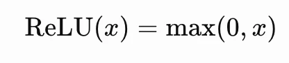
For an input of -1, ReLU returns 0. For an input of 2, it returns 2.
GELU behaves differently. An input of -1 produces approximately -0.159, while an input of 2 produces approximately 1.954.
This means GELU does not simply classify inputs as positive or negative. It applies a continuous transformation that scales different values by different amounts.
Importantly, GELU is not strictly increasing over its entire domain. Its negative region has a shallow dip before approaching zero for very negative inputs.
The Mathematics Behind GELU
The GELU activation function is defined as:
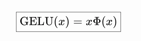
Here, Φ(x) represents the cumulative distribution function (CDF) of the standard normal distribution.
The standard normal distribution has a mean of zero and a standard deviation of one.
We can write its CDF as:
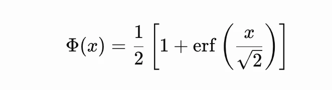
Therefore, GELU can also be expressed as:
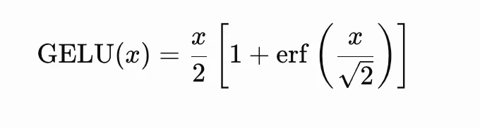
Here, erf is the error function, a mathematical function closely related to the Gaussian distribution.
A simple numerical example
Suppose a neuron receives an input of 1.
The standard normal CDF at 1 is approximately 0.8413.

Now consider an input of -1.

Notice that the positive input is mostly preserved, while the negative input is substantially reduced.
This smooth behavior is the central idea behind GELU.
Why Does GELU Use a Gaussian Distribution?
The Gaussian distribution provides a smooth way to assign weights to different input values.
For large negative inputs, the CDF approaches zero. For large positive inputs, it approaches one. At zero, its value is exactly 0.5.
Figure 2. The Gaussian CDF provides a gradual weighting factor between 0 and 1.
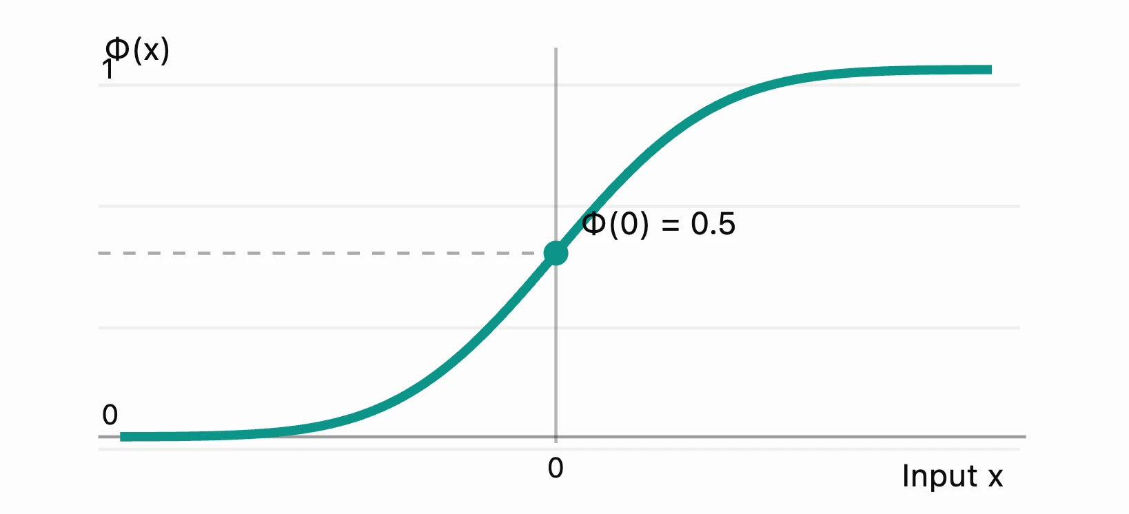
The key difference is that the Gaussian CDF acts as a scaling factor rather than a binary switch.
This is sometimes explained as a probabilistic gating mechanism. However, standard GELU is deterministic. It does not randomly remove neuron outputs during execution.
GELU vs ReLU: Key Differences
| Feature | ReLU | GELU |
|---|---|---|
| Mathematical operation | max(0, x) | x × Φ(x) |
| Negative inputs | Zeroed out | Smoothly suppressed |
| Smoothness | Not differentiable at zero | Smooth and differentiable |
| Computation | Very inexpensive | More complex |
| Output for x = 0 | 0 | 0 |
| Typical use | CNNs and lightweight MLPs | BERT-style Transformers and many MLP blocks |
| Training performance | Strong baseline | Can outperform ReLU, depending on the task |
ReLU remains popular because it is simple and computationally efficient. GELU provides a smoother transformation but requires more computation in its mathematical form.
GELU is not automatically better for every neural network. The model architecture, dataset, hardware, and implementation all affect the final result.
Why Is GELU Used in Transformers?
Transformers contain multiple components, including attention mechanisms, normalization layers, and feed-forward neural networks.
GELU is commonly used inside the feed-forward network, or FFN, rather than in the attention probability calculation itself.
A simplified Transformer feed-forward operation looks like this:

The first linear layer projects the hidden representation into another feature space. GELU introduces nonlinearity, and the second linear layer projects it back into the required hidden dimension.
In the BERT architecture, GELU is the default hidden activation, as reflected in Hugging Face’s BERT configuration.
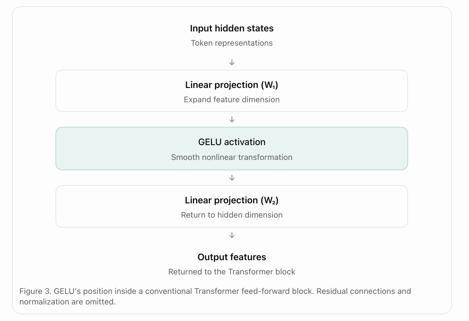
GELU also appears in vision Transformer architectures. However, not all modern language models use GELU. Some use SiLU-based gated feed-forward variants, such as SwiGLU.
The choice depends on the model architecture and its training objectives.
Approximating GELU for Efficient Computation
The exact GELU formula uses the Gaussian cumulative distribution function, which can be more computationally expensive than simpler activations.
A common approximation uses the hyperbolic tangent function:
This approximation produces values close to exact GELU while providing an alternative implementation that may be computationally efficient on certain hardware.

PyTorch supports both the exact formulation and the tanh approximation through the approximate parameter
Hands-On: Comparing GELU and ReLU Using Python
Now that we understand the theory, let’s explore how GELU behaves using Python and PyTorch.
We will first visualize both activation functions and then compare their performance on a small classification problem.
Step 1: Install the required libraries
pip install torch numpy matplotlib scikit-learnStep 2: Visualize GELU and ReLU
import torch
import torch.nn.functional as F
import matplotlib.pyplot as plt

# Generate input values
x = torch.linspace(-4, 4, 500)

# Apply activation functions
relu_output = F.relu(x)
gelu_output = F.gelu(x)

# Plot both functions
plt.figure(figsize=(9, 5))

plt.plot(x.numpy(), relu_output.numpy(),
         label="ReLU", linewidth=2)

plt.plot(x.numpy(), gelu_output.numpy(),
         label="GELU", linewidth=2)

plt.axhline(0, color="gray", linewidth=0.6)
plt.axvline(0, color="gray", linewidth=0.6)

plt.title("GELU vs ReLU Activation Functions")
plt.xlabel("Input")
plt.ylabel("Output")
plt.legend()
plt.grid(alpha=0.3)
plt.show()
The graph shows that ReLU completely removes negative values, while GELU has a smooth curve that retains some negative outputs.
Step 3: Build a simple neural network
Next, we will train two identical neural networks. One will use ReLU, and the other will use GELU.
We will use the make_moons dataset because its nonlinear decision boundary makes it useful for testing neural networks.
import numpy as np
import torch
import torch.nn as nn

from sklearn.datasets import make_moons
from sklearn.model_selection import train_test_split
from sklearn.preprocessing import StandardScaler

# Set random seed
torch.manual_seed(42)

# Generate synthetic classification data
X, y = make_moons(
    n_samples=2000,
    noise=0.25,
    random_state=42
)

# Split data into training and testing sets
X_train, X_test, y_train, y_test = train_test_split(
    X,
    y,
    test_size=0.2,
    random_state=42,
    stratify=y
)

# Normalize using training data only
scaler = StandardScaler()

X_train = scaler.fit_transform(X_train)
X_test = scaler.transform(X_test)

# Convert data into PyTorch tensors
X_train = torch.tensor(X_train, dtype=torch.float32)
X_test = torch.tensor(X_test, dtype=torch.float32)

y_train = torch.tensor(y_train, dtype=torch.long)
y_test = torch.tensor(y_test, dtype=torch.long)


# Define Neural Network
class NeuralNetwork(nn.Module):

    def __init__(self, activation):

        super().__init__()

        self.network = nn.Sequential(

            nn.Linear(2, 64),

            activation(),

            nn.Linear(64, 64),

            activation(),

            nn.Linear(64, 2)

        )

    def forward(self, x):

        return self.network(x)
Step 4: Train and compare the models
import torch
import torch.nn as nn
import torch.optim as optim
import matplotlib.pyplot as plt

def train_model(activation, epochs=100):

    torch.manual_seed(42)

    model = NeuralNetwork(activation)

    optimizer = optim.Adam(
        model.parameters(),
        lr=0.001
    )

    criterion = nn.CrossEntropyLoss()

    history = []

    for epoch in range(epochs):

        # Training phase
        model.train()

        optimizer.zero_grad()

        outputs = model(X_train)

        loss = criterion(outputs, y_train)

        loss.backward()

        optimizer.step()

        # Evaluation phase
        model.eval()

        with torch.no_grad():

            predictions = model(X_test).argmax(dim=1)

            accuracy = (
                predictions == y_test
            ).float().mean().item()

        # Store accuracy after every epoch
        history.append(accuracy)

    return model, history


# Train using ReLU activation
relu_model, relu_history = train_model(nn.ReLU)

# Train using GELU activation
gelu_model, gelu_history = train_model(nn.GELU)


# Print final accuracies
print(f"ReLU Accuracy: {relu_history[-1]:.4f}")
print(f"GELU Accuracy: {gelu_history[-1]:.4f}")


# Plot learning curves
plt.figure(figsize=(9, 5))

plt.plot(relu_history, label="ReLU")
plt.plot(gelu_history, label="GELU")

plt.xlabel("Epoch")
plt.ylabel("Test Accuracy")
plt.title("ReLU vs GELU: Learning Comparison")

plt.legend()
plt.grid(alpha=0.3)

plt.show()
Step 5: Interpret the results
After running the experiment, compare the final test accuracy and learning curves.
You might observe that GELU achieves slightly higher accuracy, converges differently, or performs similarly to ReLU. There is no guaranteed winner.
Both models have the same network architecture, optimizer, learning rate, and initialization seed. The activation function is the primary difference.
However, a single training run is not enough to establish which activation is better. For a more reliable comparison, repeat the experiment with multiple random seeds and compare the average accuracy and standard deviation. During experimentation, a validation set should be used for model selection, with the test set reserved for final evaluation.
The goal of this experiment is to understand how changing an activation function can influence model behavior, not to prove that GELU is universally superior.
Advantages and Limitations of GELU
GELU provides several useful properties, but it also introduces trade-offs.
Advantages
- Smooth activation behavior, including around zero.
- Preserves some information from moderately negative inputs.
- Fully differentiable, making gradient-based optimization straightforward.
- Successfully used in established Transformer architectures.
- Supported by major deep learning frameworks.
Limitations
- More mathematically complex than ReLU.
- May require additional computation, depending on implementation and hardware.
- Does not guarantee better accuracy or faster convergence.
- Smooth gradients do not eliminate all vanishing-gradient problems.
- May not be necessary for small or latency-sensitive models.
One important mathematical property is GELU’s derivative:
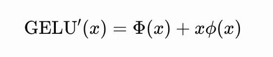
Here, Phi(x) is the standard normal probability density function.
Unlike ReLU, GELU has a derivative at zero. However, this does not mean its derivative is always positive or that gradients always remain large.
When Should You Use GELU?
GELU is a good starting point when building Transformer-style models, particularly when following an architecture that already uses it.
ReLU is still an excellent default for many conventional feed-forward networks, convolutional networks, and applications where computation cost matters.
For a pretrained model, keeping its original activation function is generally the safest choice. Replacing GELU with ReLU in a pretrained Transformer changes the model’s computations and may reduce its performance unless the modified model is appropriately retrained or fine-tuned.
In new architectures, treat the activation function as a design choice that should be evaluated experimentally.
Conclusion
GELU improves on the simple thresholding approach of ReLU by introducing smooth, input-dependent scaling. Its use of the Gaussian cumulative distribution function makes it possible to preserve small negative signals while gradually suppressing strongly negative inputs.
This behavior has made GELU an important component of several influential Transformer architectures.
However, its value is not simply that it is smoother or more mathematically sophisticated. Its practical effectiveness depends on the entire neural network, the training setup, and the hardware.
Understanding GELU provides a useful foundation for studying modern neural networks and the design decisions behind Transformer feed-forward layers.
Read more: Mamba4 Explained: A Faster Alternative to Transformers for Sequential Modeling
Frequently Asked Questions
A. ReLU acts as a hard threshold by zeroing out negative values, while GELU applies a smooth, continuous scaling based on the input’s value using a Gaussian distribution.
A. GELU provides a smoother, differentiable transformation that helps neural networks learn complex patterns more effectively, which is why it is the default in architectures like BERT.
A. The exact formula is more complex than ReLU, but developers often use a hyperbolic tangent approximation to achieve similar results with better computational efficiency on specific hardware.

Hi, I am Janvi, a passionate data science enthusiast currently working at Analytics Vidhya. My journey into the world of data began with a deep curiosity about how we can extract meaningful insights from complex datasets.
Login to continue reading and enjoy expert-curated content.

💸 Earn Instantly With This Task
No fees, no waiting — your earnings could be 1 click away.
Start Earning