Excel 101: IF, AND, OR Functions and Conditional Logic Explained

You reading this tells me you wish to learn more about Excel. This article continues our Excel series, where we explored the VLOOKUP function in the last iteration. The complete VLOOKUP guide demonstrated how the function works and how best to use it. This time, we shall bring the same focus to conditional logic and formulas like the IF function in Excel. The aim is to understand the different types of conditional logics and know how to use their operators in a working function inside Excel.

So, no fluff needed here. Let’s simply dive in, starting with what Conditional Logic in Excel is.

What is Conditional Logic in Excel?

Conditional logic in Excel means making decisions based on a condition. In simple terms, Excel checks a rule you define, evaluates the result, and then performs an action based on that outcome.

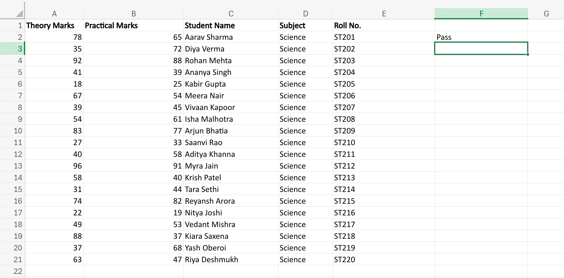
For example, suppose you have students’ marks in a sheet and want to identify whether a student has passed or failed. Rather than checking each value manually, you can simply apply a condition: if the marks are 40 or above, return “Pass”; otherwise, return “Fail”. That is conditional logic in action.

The same logic is used across many real-world tasks in Excel. You might want to mark sales above a target as “Achieved”, classify expenses as “High” or “Low”, or identify whether a payment is “Pending” or “Completed”. In each case, Excel is evaluating a condition and returning an output based on the result.

At the core of this process is a simple idea:

test a condition > get a TRUE or FALSE result > use that result to decide what happens next.

Such conditional logic is exactly what makes Excel more than just a spreadsheet for storing data. Its formulas react to values dynamically, cutting down on hours of manual work.

To make this conditional logic work, Excel relies on conditional operators, which are the symbols used to compare values. Next, let us learn about conditional operators in detail.

Also read: 50+ Excel Interview Questions to Ace Your Interview

What are Conditional Operators in Excel?

Think about it, how exactly will you compare values inside Excel for any conditional logic to work? You will need comparison symbols for different conditions, like equal (=), greater than (>), smaller than (<), etc., right? All such comparison symbols are called conditional operators in Excel. In essence, these are used to test whether a condition is true or false. They are the building blocks behind conditional logic, because they allow Excel to compare values before a function decides what to return.

In simple terms, these operators help Excel answer questions like:

• Is this value greater than 50?
• Is this cell equal to “Yes”?
• Are these two values different?
• Has the target been met or not?

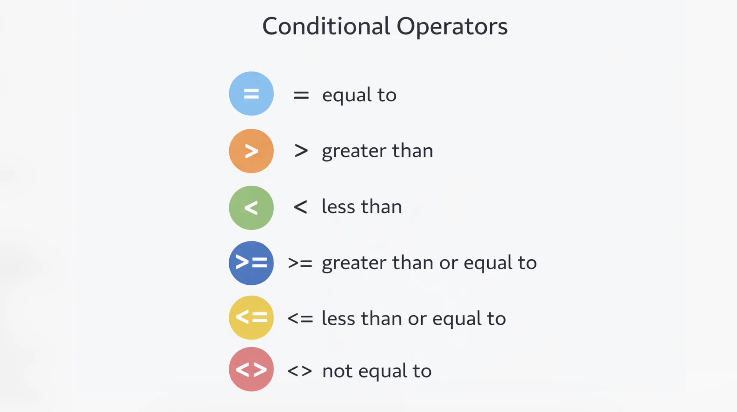
Excel supports six main conditional operators:

• `=` : equal to
• `>` : greater than
• `<` : less than
• `>=` : greater than or equal to
• `<=` : less than or equal to
• `<>` : not equal to

Let us understand this with a simple example. Suppose cell `A2` contains the value `75`.

=A2>50

Excel checks whether 75 is greater than 50. Since that condition is true, the formula returns `TRUE`.

Now look at this:

=A2<50

This time, Excel checks whether 75 is less than 50. Since that is not true, the result is `FALSE`.

That `TRUE` or `FALSE` output is what powers conditional formulas in Excel. Functions like `IF`, `IFS`, `AND`, and `OR` rely on these comparisons to make decisions.

For example:

=IF(A2>=40,"Pass","Fail")

Don’t worry, we will learn about the IF function in detail shortly. For now, just note in this example that Excel first checks whether the value in `A2` is greater than or equal to 40. If the condition is true, it returns `Pass`. If the condition is false, it returns `Fail`. More importantly, note that even the IF function begins with a conditional operator.

So, while functions like `IF` often get all the attention, the real decision-making starts with these operators. They are what tell Excel how to evaluate a condition in the first place.

Now that the operators are clear, the next step is to understand the conditional functions in which they are used, starting with the `IF` function.

Also read: Microsoft Excel for Data Analysis

IF Function in Excel

The IF function is one of the most widely used formulas in Excel. In its most basic sense, it checks whether a condition is true or false, and then returns a result based on that outcome. In simple words, it tells Excel: if this happens, do this; otherwise, do that.

To understand it properly, let us break it into two parts.

IF Function Syntax

The syntax of the IF function is:

=IF(logical_test, value_if_true, value_if_false)

Here, each part has a specific role:

• logical_test is the condition Excel checks
• value_if_true is the result returned if the condition is true
• value_if_false is the result returned if the condition is false

Let us look at a simple example:

=IF(A2>=40,"Pass","Fail")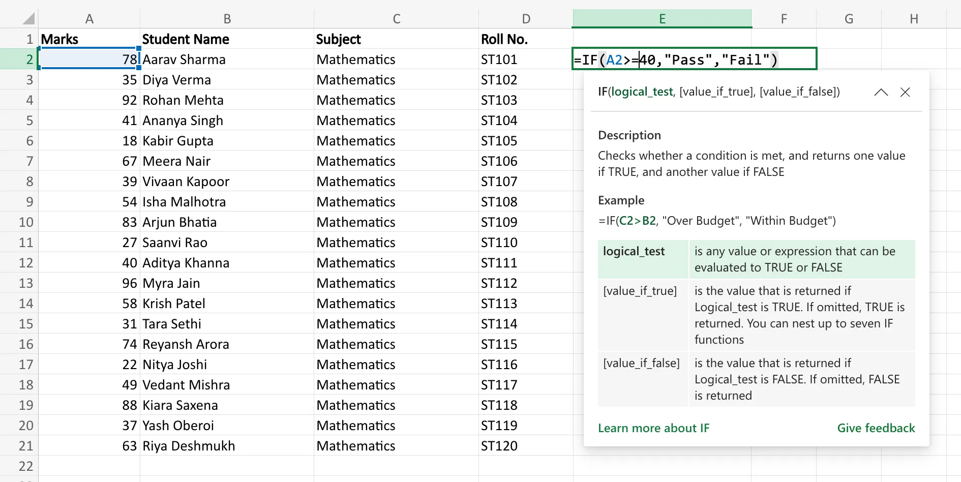

Here is what Excel is doing in this formula:

• It first checks whether the value in cell A2 is greater than or equal to 40
• If that condition is true, Excel returns Pass
• If that condition is false, Excel returns Fail

So, if A2 contains 65, the result will be Pass. If it contains 28, the result will be Fail.

This is the basic structure of every IF formula. First, Excel evaluates the condition. Then it decides which result to return.

Forming the Formula

Now that the syntax is clear, the next step is to actually build the formula in Excel.

Suppose you have marks listed in column A, and you want to show the result in column B.

Start by clicking the cell where you want the output to appear. Then type:

=IF(A2>=40,"Pass","Fail")

Press Enter, and Excel will instantly return the result based on the value in A2.

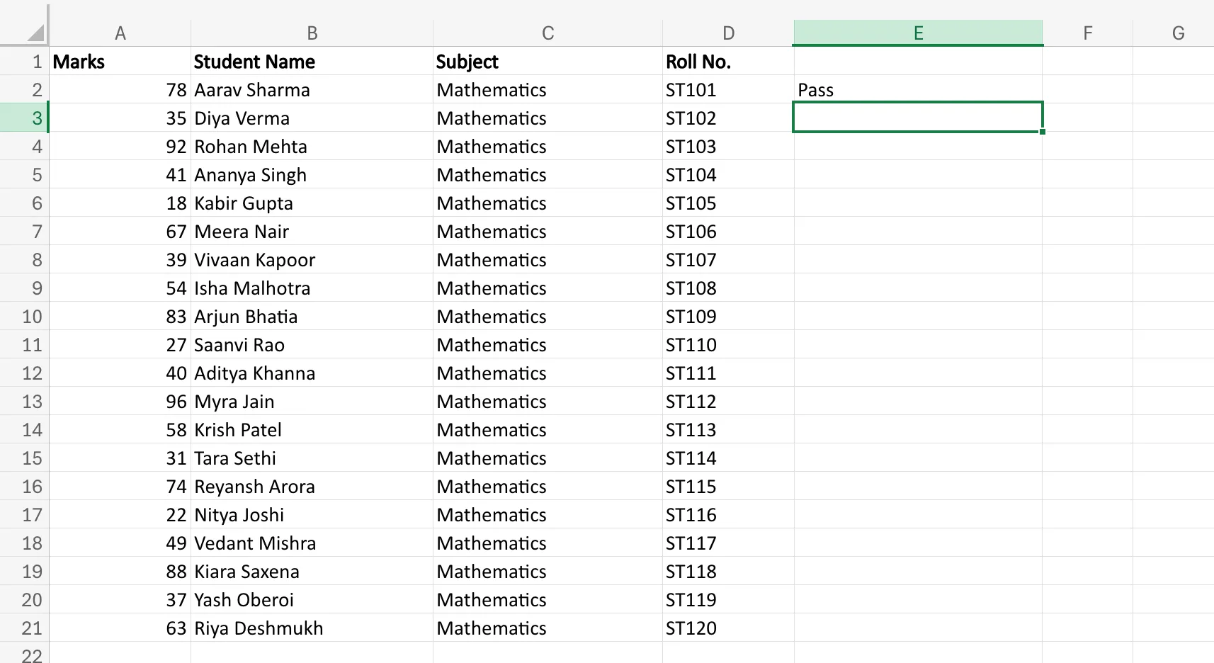
Since the value meets the condition in this case, you get ‘Pass’. If it did not, you would get ‘Fail’.

Once the formula works in one cell, you can drag it down to apply the same logic to the rest of the rows. Excel will automatically adjust the cell reference for each row.

For instance:

• in row 2, Excel checks A2
• in row 3, it checks A3
• in row 4, it checks A4

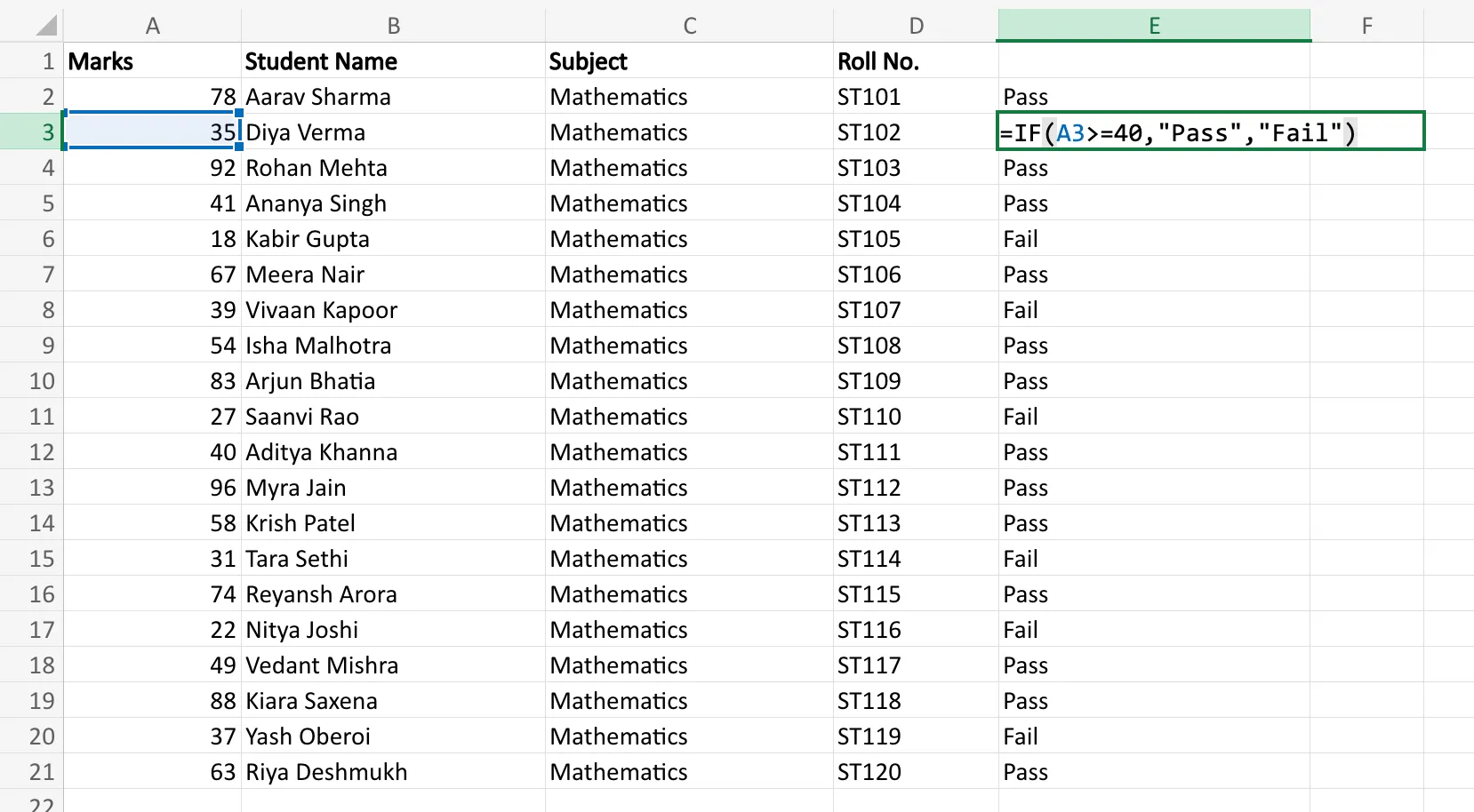
This is what makes the IF function so useful. You create the logic once, and Excel repeats it across the dataset in seconds.

Now that we understand how a single IF formula works, the next step is to see what happens when there are more than two possible outcomes. That is where Nested IF statements come in.

Nested IF Statements in Excel

A single `IF` function works well when there are only two outcomes. But many real Excel tasks involve more than just a yes-or-no decision. You may need to assign grades, label performance bands, or categorise values into multiple groups. That is where Nested IF statements come in.

A Nested IF simply means placing one `IF` function inside another, so Excel can test multiple conditions one after the other.

Nested IF Syntax

Consider a simple Excel sheet that has the marks of students stored as data, and you have to grade the students based on their marks. A basic Nested IF formula for the same will look something like this:

=IF(A2>=90,"A",IF(A2>=75,"B",IF(A2>=40,"C","Fail")))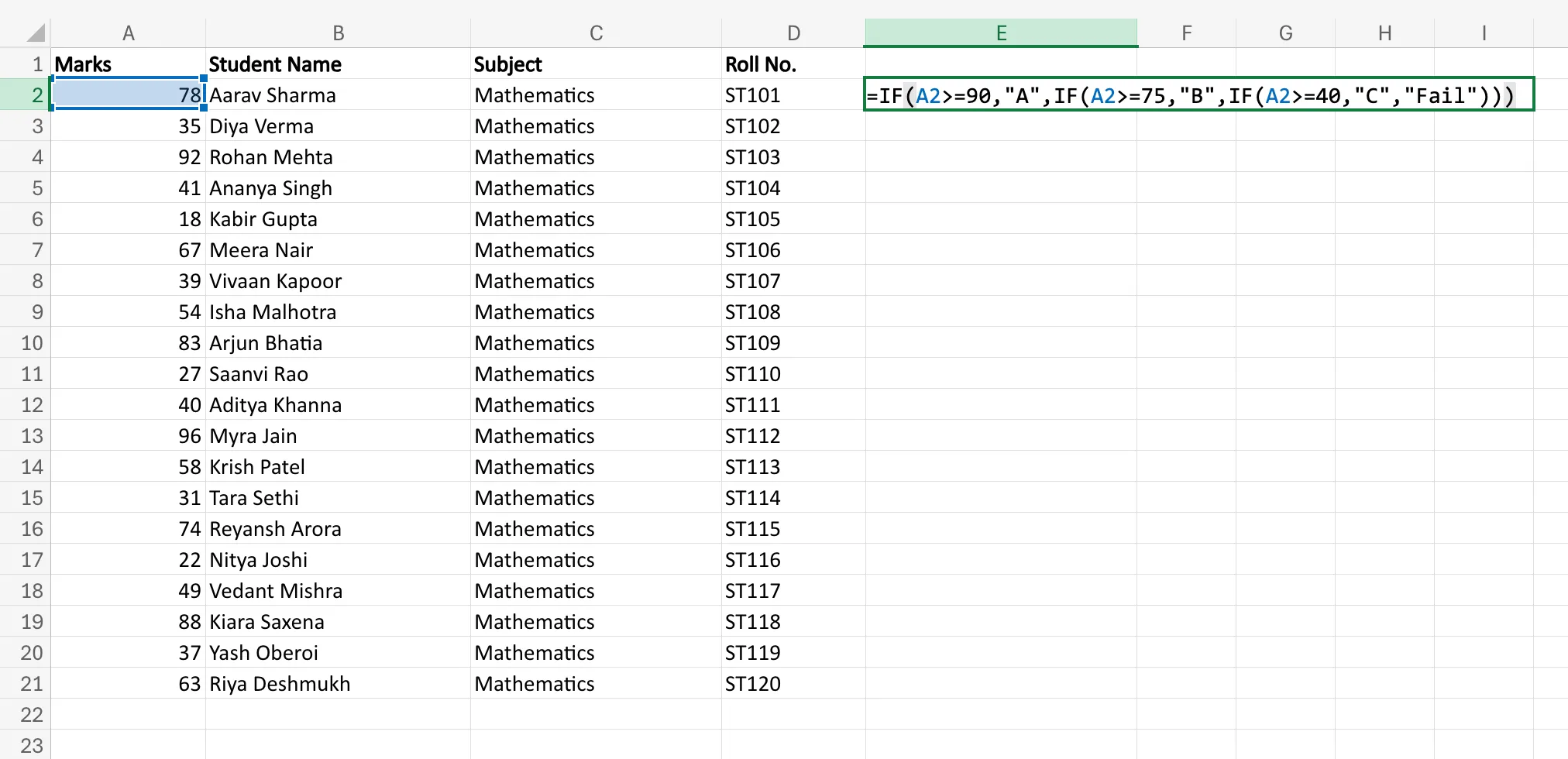

This may look intimidating at first, but the logic is straightforward. Excel checks each condition in sequence:

• If `A2` is 90 or above, it returns `A`
• If not, it checks whether `A2` is 75 or above, and returns `B`
• If not, it checks whether `A2` is 40 or above, and returns `C`
• If none of these conditions are met, it returns `Fail`

So if `A2` contains 82, the formula returns `B`. If it contains 36, Excel returns `Fail`.

The key thing to understand here is that Excel stops as soon as it finds the first true condition. It does not keep checking the rest.

Forming the Formula

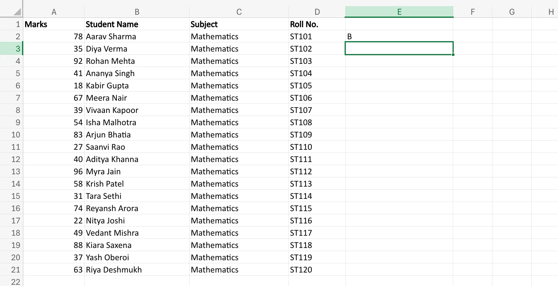
Suppose you have student marks in column `A`, and you want to assign grades in column `B`.

Click the output cell and enter:

=IF(A2>=90,"A",IF(A2>=75,"B",IF(A2>=40,"C","Fail")))

Then press Enter.

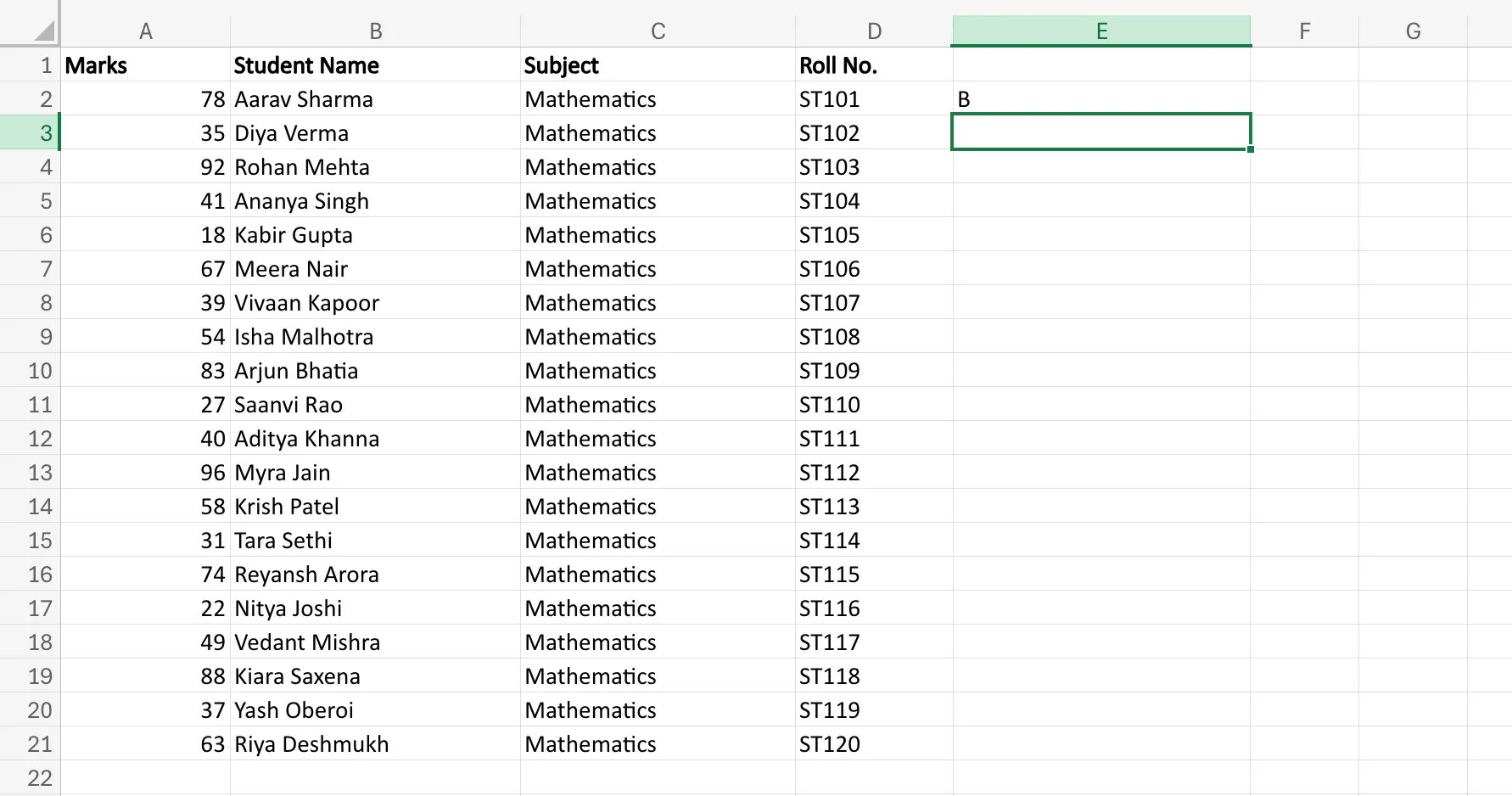
Excel will evaluate the conditions from left to right and return the correct grade for that row. Once the formula works, drag it down to apply the same grading logic to the rest of the data, as seen in the image below.

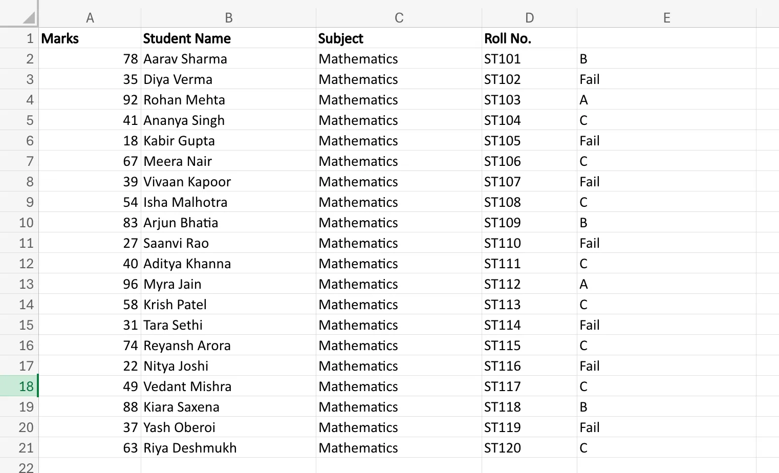
One important thing to remember: the order of conditions matters. In the example above, the highest score range is checked first. If you reverse the order carelessly, Excel may return the wrong result.

Nested IF statements are useful, but they can become difficult to read when too many conditions are involved. That is exactly why Excel introduced a cleaner alternative called `IFS`.

Also read: 10 Most Commonly Used Statistical Functions in Excel

IFS Function in Excel

Imagine if, in the grading example above, you had grades up to Z to hand out. The Nested `IF` statements may get the job done, but will definitely become very messy, very quickly. Once you start stacking multiple conditions inside one another, the formula becomes harder to read, harder to edit, and easier to break. That is where the `IFS` function helps.

The `IFS` function is designed to test multiple conditions in a cleaner format. Instead of nesting one `IF` inside another, you list each condition and its result in sequence.

IFS Function Syntax

The syntax of the `IFS` function is:

=IFS(logical_test1, value_if_true1, logical_test2, value_if_true2, ...)

Each logical test is followed by the result Excel should return when that condition is true.

Let us take the same grading example we used in Nested IF:

=IFS(A2>=90,"A",A2>=75,"B",A2>=40,"C",A2<40,"Fail")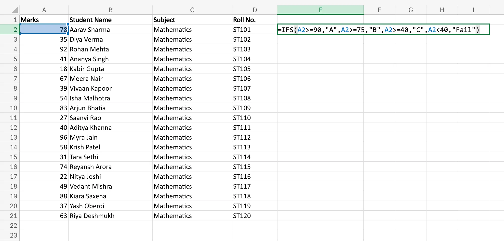

Here is what Excel does:

• If `A2` is 90 or above, it returns `A`
• If not, it checks whether `A2` is 75 or above, and returns `B`
• If not, it checks whether `A2` is 40 or above, and returns `C`
• If `A2` is below 40, it returns `Fail`

The logic is similar to Nested IF, but the structure is much cleaner. You do not have to keep track of multiple closing brackets inside brackets.

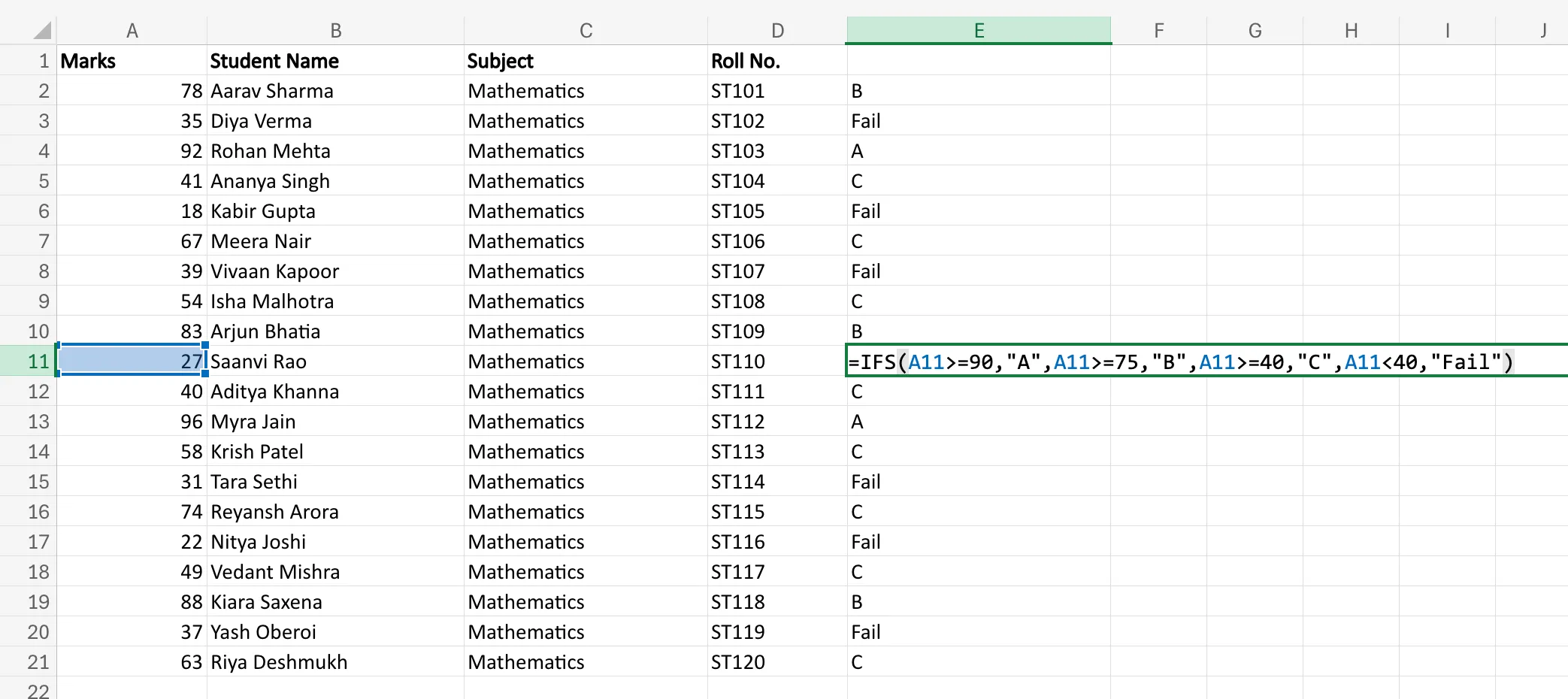
Forming the Formula

Suppose marks are listed in column `A`, and you want grades in column `B`.

Click the output cell and type:

=IFS(A2>=90,"A",A2>=75,"B",A2>=40,"C",A2<40,"Fail")

Then press Enter.

Excel will test the conditions in order and return the result for the first condition that evaluates to true. After that, you can drag the formula down for the rest of the rows.

This makes `IFS` especially useful when you have several possible outcomes and want the formula to stay readable.

That said, `IFS` is best when you are checking multiple separate conditions. But sometimes the challenge is not multiple outcomes. Sometimes you want to test more than one condition at the same time. For that, Excel uses `AND` and `OR` functions.

AND and OR Functions in Excel

So far, we have looked at formulas where Excel checks one condition at a time. But in real spreadsheets, a single condition is often not enough. You may want a result only when multiple conditions are true, or when at least one out of several conditions is true. This is where `AND` and `OR` come in.

Both are logical functions in Excel, and they are usually used inside formulas like `IF`.

AND Function Syntax

The `AND` function returns `TRUE` only when all conditions are true.

Its syntax is:

=AND(logical1, logical2, ...)

Let us say a student passes only if they score more than 40 in theory and more than 40 in practical.

=AND(A2>40,B2>40)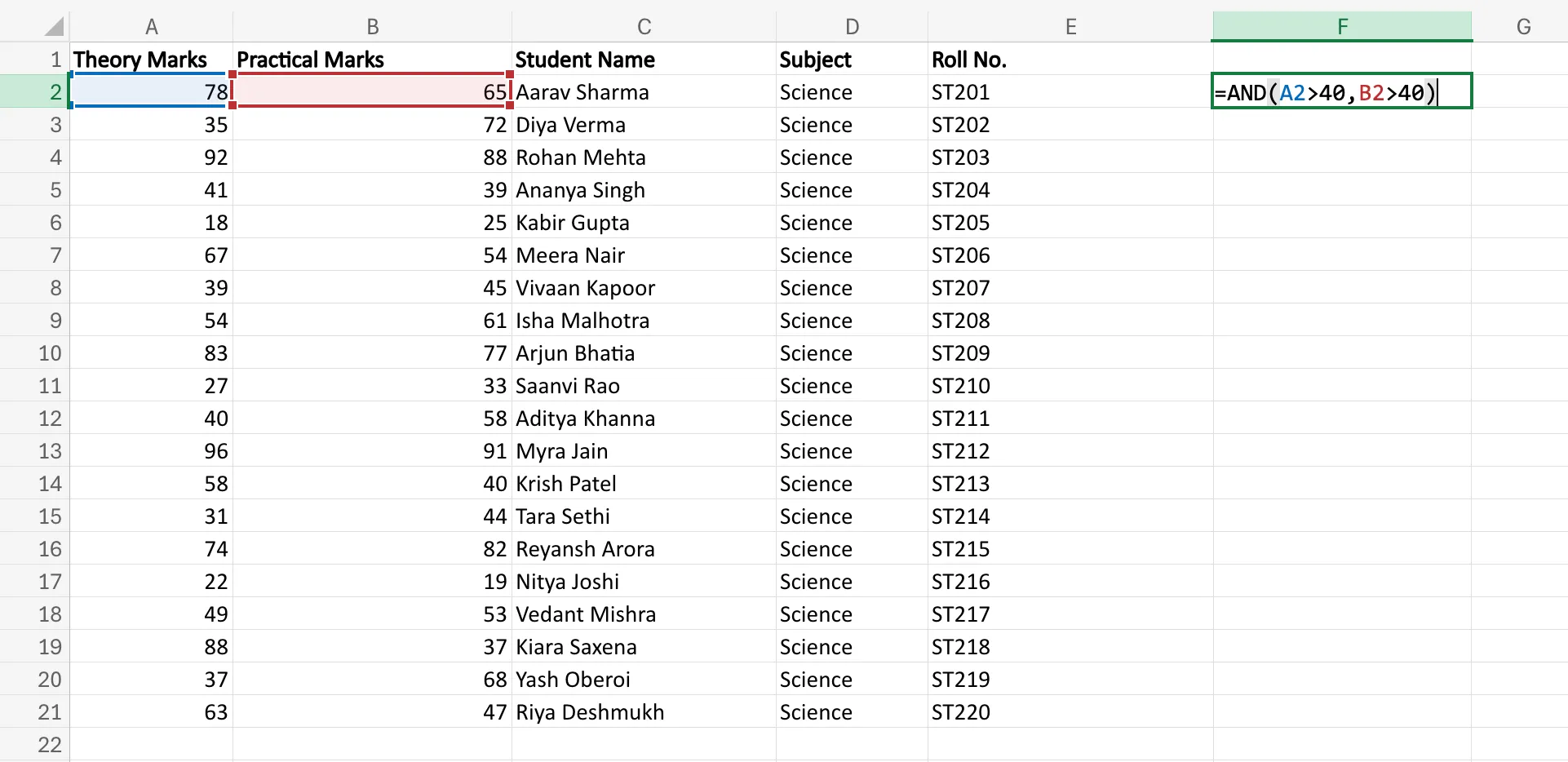

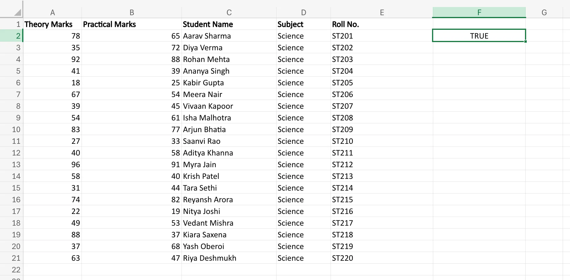
Here, Excel checks both conditions:

• Is `A2` greater than 40?
• Is `B2` greater than 40?

If both are true, Excel returns `TRUE`. If even one is false, Excel returns `FALSE`.

Now let us use it inside an `IF` function:

=IF(AND(A2>40,B2>40),"Pass","Fail")

This tells Excel to return Pass only if both conditions are satisfied. Otherwise, it returns Fail.

OR Function Syntax

The `OR` function works differently. It returns `TRUE` when at least one condition is true.

Its syntax is:

=OR(logical1, logical2, ...)

Suppose a salesperson qualifies for a bonus if they either cross a sales target or bring in a new client.

=OR(A2>=100000,B2="Yes")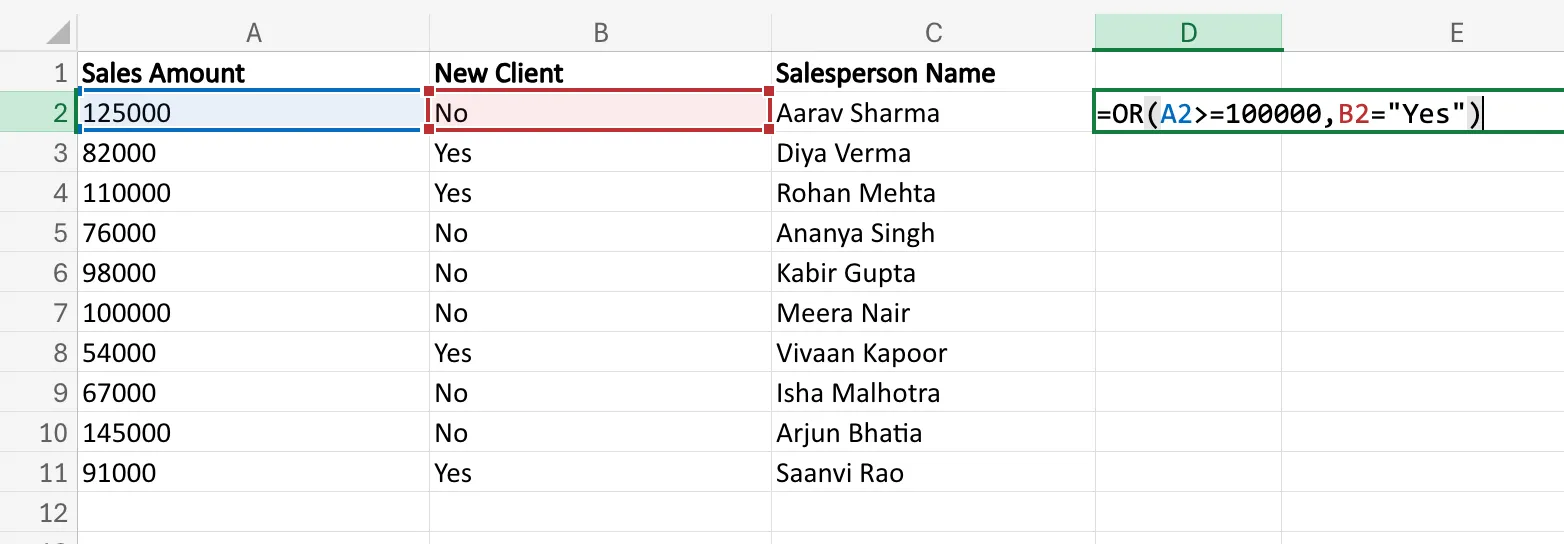

Here, Excel checks:

• Is `A2` greater than or equal to 100000?
• Is `B2` equal to “Yes”?

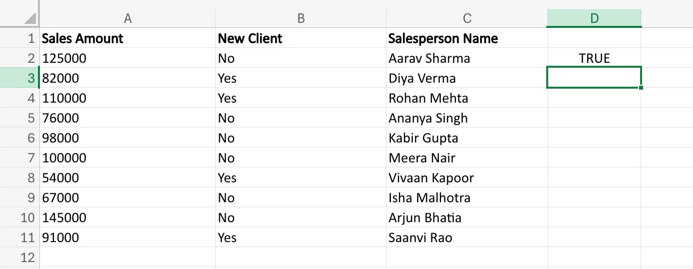
If even one of these is true, Excel returns `TRUE`.

Used inside `IF`, it becomes:

=IF(OR(A2>=100000,B2="Yes"),"Bonus Eligible","Not Eligible")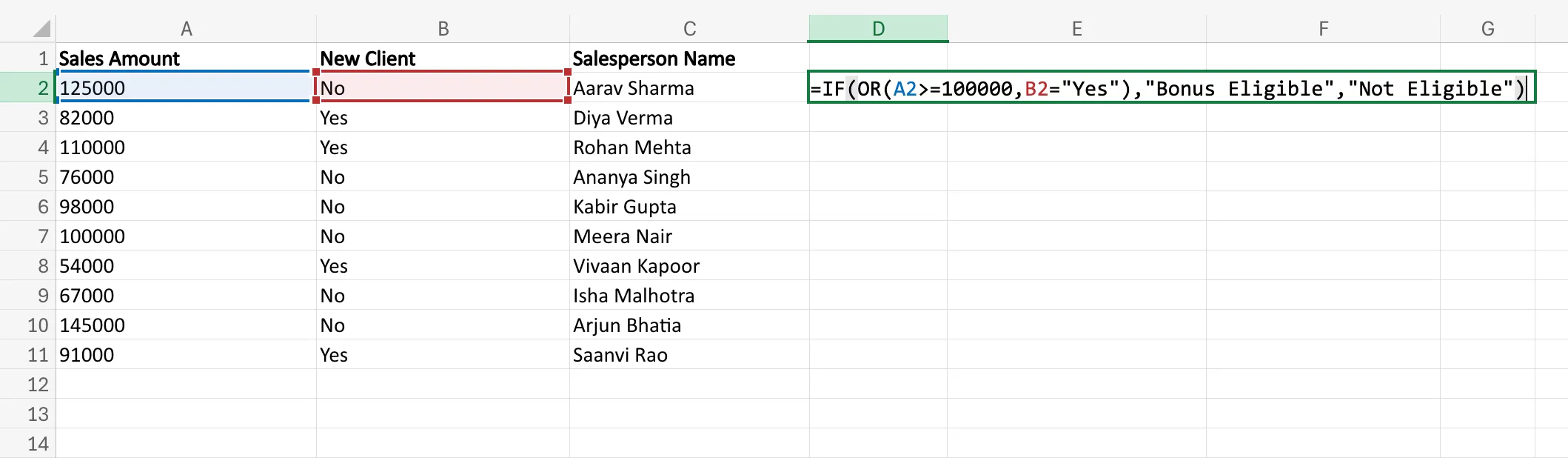

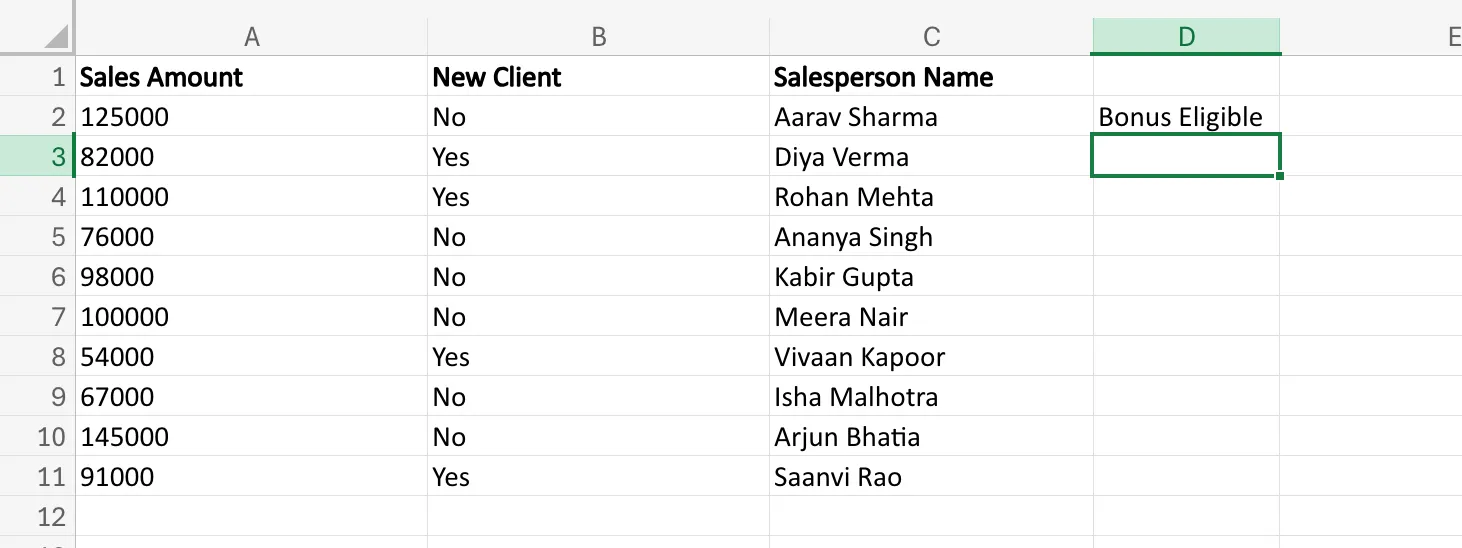
So if the person meets either one of the conditions, Excel marks them as Bonus Eligible.

Forming the Formula

The easiest way to build these formulas is to first decide your logic clearly.

• Use `AND` when every condition must be met.
• Use `OR` when just one condition is enough.

For example, if an employee gets approval only when they have completed training and submitted documents, you would write:

=IF(AND(A2="Yes",B2="Yes"),"Approved","Pending")

But if they can qualify through either of two routes, you would use:

=IF(OR(A2="Yes",B2="Yes"),"Approved","Pending")

That is the core difference. `AND` is stricter. `OR` is more flexible.

These functions become especially powerful when combined with `IF`, because they allow Excel to handle more realistic decision-making rules. But even then, formulas can still break if the data throws an error. That is where `IFERROR` and `IFNA` become useful.

IFERROR and IFNA in Excel

Even when your logic is correct, Excel formulas do not always return clean results. Sometimes they produce errors because a value is missing, a lookup fails, or the formula cannot process the input. That is where `IFERROR` and `IFNA` become useful.

These functions help you replace ugly error messages with something more meaningful and readable. Instead of showing `#VALUE!`, `#DIV/0!`, or `#N/A`, you can ask Excel to return a custom output.

IFERROR Function Syntax

The `IFERROR` function checks whether a formula returns any error. If it does, Excel shows the value you specify instead.

Its syntax is:

=IFERROR(value, value_if_error)

Here:

• `value` is the formula or expression Excel should evaluate
• `value_if_error` is what Excel should return if the formula results in an error

Let us look at an example:

=IFERROR(A2/B2,"Error in Calculation")

Here, Excel tries to divide `A2` by `B2`.

• If the division works, Excel returns the actual result
• If the formula throws an error, such as division by zero, Excel returns Error in Calculation

This is useful because it keeps your worksheet cleaner and easier to understand.

Forming the IFERROR Formula

Suppose you are calculating percentage growth, and there is a chance that the previous value is zero. A normal division formula may return an error. To avoid that, you can wrap the formula inside `IFERROR`:

=IFERROR((B2-A2)/A2,"Not Available")

Press Enter, and Excel will either show the growth value or return **Not Available** if the formula breaks.

This helps a lot in reports and dashboards, where error values can make the sheet look messy or confusing.

IFNA Function Syntax

The `IFNA` function is more specific. It only handles the `#N/A` error, which usually appears when a lookup formula cannot find a match.

Its syntax is:

=IFNA(value, value_if_na)

Let us take a simple example with `VLOOKUP`:

=IFNA(VLOOKUP(E2,A2:C10,2,FALSE),"Not Found")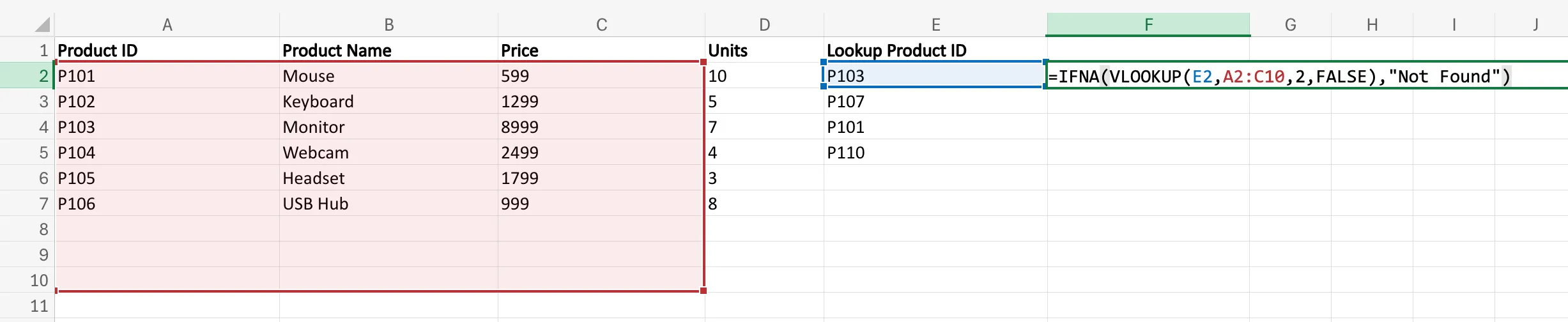

Here, Excel tries to find the value from `E2` inside the range `A2:C10`.

• If a match is found, it returns the corresponding result
• If no match is found and Excel produces `#N/A`, it returns Not Found

This is better than showing `#N/A` to the reader, especially in lookup-based sheets.

Forming the IFNA Formula

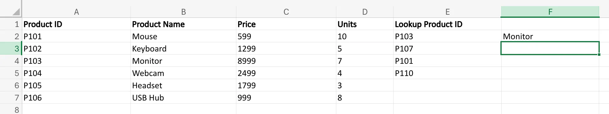
Suppose you have a product ID in cell `E2`, and you want to fetch the product name from a lookup table. If the ID does not exist, you do not want Excel to show an error.

So instead of writing only:

=VLOOKUP(E2,A2:C10,2,FALSE)

you can write:

=IFNA(VLOOKUP(E2,A2:C10,2,FALSE),"Product Not Found")

This makes the output much more user-friendly.

IFERROR vs IFNA

The difference is simple:

• `IFERROR` handles all types of errors
• `IFNA` handles only the `#N/A` error

So if you are dealing with lookups and only want to catch missing matches, `IFNA` is more precise. But if you want a broader safety net for any error, `IFERROR` is the better choice.

At this point, we have covered the key Excel functions that power conditional logic: `IF`, Nested `IF`, `IFS`, `AND`, `OR`, `IFERROR`, and `IFNA`. The final step is to bring everything together with a practical conclusion on when to use each one.

Also read: Advanced Excel for Data Analysis

Conclusion

As you start using these formulas in your Excel sheets more often, you will realise the amount of time each of these can save you. These functions are what make Excel feel like a working decision system. Instead of just storing numbers and text, Excel can evaluate conditions, apply rules, and return the right answers automatically. Hence, these formulas like `IF`, `IFS`, `AND`, `OR`, `IFERROR`, and `IFNA` have so much practical value.

To sum up, the `IF` function is the starting point when you need Excel to choose between two outcomes. Nested `IF` helps when those outcomes increase. `IFS` offers a cleaner way to handle multiple conditions without turning the formula into a bracket jungle. `AND` and `OR` take the logic further by allowing you to test multiple conditions together, depending on whether all or just one of them needs to be true. Finally, `IFERROR` and `IFNA` help make your spreadsheets more readable by replacing error messages with useful outputs.

Since they have such high practical value, the real benefit of learning these functions is the ability to make spreadsheets smarter, cleaner, and far more useful in real work. Once you understand how conditional logic works, you realise the power of Excel when it comes to interpreting data.